A How to efficientnet Keras Classification

Humans, unlike computers, make sense of what they see based on their experiences, memories, and biological structure. The human brain extracts and analyzes humongous volumes of data using visual cues. To understand the true effect of sight, 40% of our nerve fibers are linked to the retina, and 90% of the information transmitted to the brain is visual. In fact, research at 3M Corporation concluded that we process visuals 60,000 times faster than text.

Computer Vision Tasks with EfficientNet Keras Classification

To begin with, image classification is a fundamental task that assesses an entire image. The goal is to classify the image by assigning it a specific label. Typically, image classification refers to images in which only one object appears and which a computer analyzes. Besides, object detection involves both classification and localization tasks, and analyzes more realistic cases in which multiple objects may exist in an image. In general, there are two methods of classification: supervised and unsupervised.

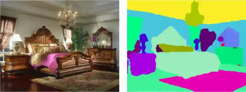
Furthermore, the more advanced task of separating pixels in an image to a particular object or class requires computer vision techniques and methods. Data scientists and computer vision specialists refer to such tasks as "semantic segmentation" or "dense prediction." Semantic segmentation is particularly popular in autonomous vehicles such as cars, drones, and planes, in addition to medical image diagnosis.

Computer Vision Tasks with efficientnet Keras classification

In this post, we will discuss convolutional neural networks, data augmentation, EfficientNet, and how to achieve nearly 100% accuracy on a classification of several classes of images potentially across multiple datasets. Understanding Deep Convolutional Neural Networks (ConvNets or CNNs) are at the center of computer vision and in my view, deep learning applications.

Convolutional Neural Networks

Convolutional neural networks (CNNs) are the most popular neural network for image classification. Comparing to a fully connected neural network, fewer parameters in CNN greatly improve the training time as well as reduce the amount of sufficient data. Instead of a fully connected network of weights for each pixel, a CNN can process a small patch of the image for a prediction.

Consider an image; a CNN can efficiently scan it chunk by chunk—for instance, in a 5 by 5 window. The 5-by-5 window slides along the image (usually from left to right and top to bottom). How quickly it slides is called its stride length. For example, a stride length of 2 means the 5 by 5 sliding window moves by 2 pixels at a time until it covers the entire image.

A convolution is a weighted sum of the pixel values of the image as the window slides across the whole thing.

Turns out, this convolution process throughout an image with a weight matrix produces another image.

The sliding-window operations occur in the convolution layer of the neural network. In general, a CNN has multiple convolutional layers. Each convolutional layer typically generates many alternate convolutions, so the weight matrix is a tensor of 5 by 5 by n, where n is the number of convolutions.

As an example, let’s say an image goes through a convolution layer on a weight matrix of 5 by 5 by 64. It generates 64 convolutions by sliding a 5 by 5 window. Therefore, this model has 5 by 5 by 64 = 1,600 parameters, which is remarkably fewer parameters than a fully connected network: 256 by 256 = 65,536.

More often than not, image classification datasets are significant in size. Nevertheless, we use data augmentation in order to further generalize the model. is the process of generating additional training data from your existing examples by augmenting them using random transformations that yield similar-looking images. This exposes the model to more aspects of the data and prevents over-fitting.

According to the documentation of , we can combine the data augmentation, rescaling, and the CNN model in this manner: Data Augmentation Pipeline for EfficientNet Classification

model = Sequential([
  data_augmentation,
  layers.experimental.preprocessing.Rescaling(1./255),
  layers.Conv2D(16, 3, padding='same', activation='relu'),
  layers.MaxPooling2D(),
  layers.Conv2D(32, 3, padding='same', activation='relu'),
  layers.MaxPooling2D(),
  layers.Conv2D(64, 3, padding='same', activation='relu'),
  layers.MaxPooling2D(),
  layers.Dropout(0.2),
  layers.Flatten(),
  layers.Dense(128, activation='relu'),
  layers.Dense(num_classes)
])

Data Augmentation Pipeline for efficientnet classification

In general, we can also divide the process of image augmentation into four steps regardless of the neural network architecture:

Import libraries and images.
Define an augmentation pipeline.
Read images.
Pass images to the augmentation pipeline and receive augmented images.

For reading images from disk and resizing them, we can use OpenCV. Meanwhile, for data augmentation is a fast and flexible library compatible with different neural networks.

An example of data augmentation in albumenations is: horizontal flips with a probability of 50%; rotation by a random angle in the range of 0 to 15 degrees with a probability of 50%; either sharpening or embossing the input image with 50%/3=16.67%; embossing the image with 16.67%; or randomly changing brightness and contrast with 16.67%; and cutting out five holes in 50% of instances.

def augment_image(image):
    aug = A.Compose([
        A.HorizontalFlip(p=0.5),
        A.Rotate(limit=[0, 15], p=0.5),
        A.OneOf([
            A.IAASharpen(),
            A.IAAEmboss(),
            A.RandomBrightnessContrast(),
        ], p=0.5),
        A.Cutout(num_holes=5, max_h_size=20, max_w_size=20, fill_value=0, always_apply=False, p=0.5)
    ])
    augmented = aug(image=image)
    return augmented['image']

The following class reads images, resizes them, augments them, and passes the batch size to our neural network.

class CustomDataGen(tf.keras.utils.Sequence):
    def __init__(self, df,
                 augment=True,
                 batch_size=8,
                 input_shape=(224, 224, 3),
                 shuffle=True):
        self.paths = df.path.values
        self.labels = df.target.values
        self.augment = augment
        self.batch_size = batch_size
        self.input_shape = input_shape
        self.shuffle = shuffle
        self.n = len(self.paths)
        self.on_epoch_end()
    def on_epoch_end(self):
        self.indexes = np.arange(len(self.paths))
        if self.shuffle == True:
            np.random.shuffle(self.indexes)
    def __load_data(self, paths, labels):
        X_batch = []
        y_batch = []
        for path, label in zip(paths, labels):
            X = cv2.imread(path).copy()
            X = cv2.cvtColor(X, cv2.COLOR_BGR2RGB)
            X = cv2.resize(X, (self.input_shape[0], self.input_shape[1]))
            if self.augment:
                X = augment_image(X)
            X_batch.append(X / 255.)
            y = np.zeros((5))
            y[label] = 1
            y_batch.append(y)
        return np.array(X_batch, dtype=float), np.array(y_batch, dtype=float)
    def __getitem__(self, index):
        indexes = self.indexes[index*self.batch_size:(index+1)*self.batch_size]
        X, y = self.__load_data([self.paths[i] for i in indexes],
                                [self.labels[i] for i in indexes])
        return X, y
    def __len__(self):
        return int(np.floor(len(self.paths) / self.batch_size))

efficientnet Keras classification

EfficientNet is a state-of-the-art convolutional neural network that Google released as open source. A family of image classification models achieves state-of-the-art accuracy yet is an order of magnitude smaller and faster than previous models such as and .

def create_model(input_shape=(224, 224, 3)):
    inputs = Input(input_shape)
    base_model = EfficientNetB1(input_shape=input_shape, include_top=False, classes=5)
    x = base_model(inputs)
    x = GlobalAveragePooling2D()(x)
    x = Dense(256, activation='relu')(x)
    x = Dropout(0.1)(x)
    outputs = Dense(5, activation='softmax')(x)
    model = Model(inputs, outputs)
    return model

model = create_model((224, 224, 3))
metrics = [
'accuracy',
'AUC'
]

model.compile(optimizer=Adam(), loss='categorical_crossentropy', metrics=metrics)
model.summary()

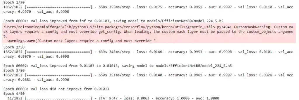
Combining the functions and classes

Finally, we combine the augmentation pipeline, the data generator and our model to estimate the class of the image. On the fourth epoch the model reaches 100%. On the withheld dataset the model generated comparable 99.6%.

Summary

In this post, we discussed convolutional neural networks, data augmentation, EfficientNet, and how to achieve nearly 100% accuracy on a classification of several classes of images. Data scientists and computer vision specialists refer to such tasks as "semantic segmentation" or "dense prediction." Semantic segmentation is a particularly popular term in autonomous vehicles such as cars, drones, and planes. The sliding-window operations occur in the convolution layer of the neural network. A convolution is a weighted sum of the pixel values of the image, as the window slides across the whole thing.

Data augmentation is the process of generating additional training data from your existing examples. This exposes the model to more aspects of the data and prevents over-fitting. In this example, we are using Google Brain's EfficientNet family of image classification models, which are an order-of-magnitude smaller and faster than previous models such as ResNet-152 and Resnet-50. Albumentations is a fast and flexible library compatible with different neural networks.