How to implement Realized Volatility python

Volatility estimators are especially valuable in modelling financial returns and capturing time-variability of financial series.

In this article, we discuss advanced metrics of volatility and measures of integrated quarticity. Besides, we implement the estimators in Pandas, NumPy and SciPy python libraries.

Quarticity and Realized Volatility python

The libraries that we are using in the implementation of the math formulas are

from scipy.special import gamma
import numpy as np
import pandas as pd

Furthermore, we estimate additional volatility estimators that we build upon realized quarticity, realized quad-power quarticity and realized tri-power quarticity.

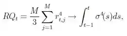
The realized fourth-power variation or realized quarticity is a consistent estimator of the integrated quarticity

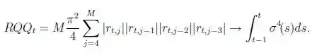
A more robust estimator, particularly in the presence of jumps, is the realized quad-power quarticity

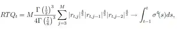
Similarly robust estimator is also the realized tri-power quarticity

In python an implementation looks as following

def realized_quarticity(series):
    series = np.log(series).diff()
    return np.sum(series**4)*series.shape[0]/3
df.groupby(df.index.date).agg(realized_quarticity)

python numpy realized quarticity estimator

def realized_quadpower_quarticity(series):
    series = np.log(series).diff()
    series = abs(series.rolling(window=4).apply(np.product, raw=True))
    return (np.sum(series) * series.shape[0] * (np.pi**2))/4
df.groupby(df.index.date).agg(realized_quadpower_quarticity)

python numpy realized quadpower quarticity estimator

def realized_tripower_quarticity(series):
    series = np.log(series).diff() ** (4/3)
    series = abs(series).rolling(window=3).apply(np.prod, raw=True)
    return series.shape[0]*0.25*((gamma(1/2)**3)/(gamma(7/6)**3))*np.sum(series)
df.groupby(df.index.date).agg(realized_quadpower_quarticity)

python numpy realized tripower quarticity estimator

Moreover, these estimates assist in estimation of three additional realized volatility estimators:

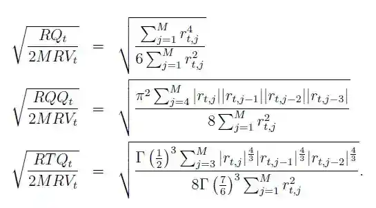
def realized_1(series):
    series = np.log(series).diff()
    return np.sqrt(np.sum(series**4)/(6*np.sum(series**2)))
df.groupby(df.index.date).agg(realized_1)

python numpy realized volatility estimator 1

def realized_2(series):
    series = np.log(series).diff()
    return np.sqrt(((np.pi**2)*np.sum(abs(series.rolling(window=4).apply(np.product, raw=True))))/(8*np.sum(series**2)))
df.groupby(df.index.date).agg(realized_2)

python numpy realized volatility estimator 2

def realized_3(series):
    series = np.log(series).diff()
    numerator = (gamma(1/2)**3)*np.sum((abs(series)**(4/3)).rolling(window=3).apply(np.prod))
    denominator = 8 * (gamma(7/6)**3)*np.sum(series**2)
    return np.sqrt(numerator/denominator)
df.groupby(df.index.date).agg(realized_3)

python numpy realized volatility estimator 3

Further ideas to explore

Corsi et al. (2008) research paper suggests that we can optimize our strategy by taking into account residuals from GARCH model. In particular, they demonstrate that the residuals of the commonly used time–series models for realized volatility exhibit non–Gaussian properties and volatility clustering. To accommodate these properties, authors extend models for realized volatility by replacing the Gaussian with the more flexible normal inverse Gaussian (NIG) distribution to allow for fat–tails and skewness.

From this paper we also reference the idea of less well-known time-series model, auto-regressive fractionally integrated moving average (ARFIMA), which they claimed in 2005 was a promising strategy for modeling and predicting volatility.

Additionally, we might include current and lagged variables as proxies for the information arrival process which potentially can add insight on future volatility.

Finally, we can explicitly separate quadratic variation into continuous and jump components in order to increase the robustness.

Conclusion

Realized Volatility python is a metric that helps to measure the time-variability of financial series. It is used to measure the volatility of returns and capture the time-variability of financial series. In this article, we discussed advanced metrics of volatility and measures of integrated quarticity. We implemented the estimators in Pandas, NumPy and SciPy python libraries. We discussed the realized fourth-power variation or realized quarticity, realized quad-power quarticity, and realized tri-power quarticity. We also discussed additional volatility estimators such as realized volatility estimator 1, realized volatility estimator 2, and realized volatility estimator 3. Furthermore, we discussed ideas to explore such as the use of residuals from GARCH model, the use of ARFIMA model, the use of current and lagged variables as proxies for the information arrival process, and the separation of quadratic variation into continuous and jump components.

Quarticity and Realized Volatility python

Further ideas to explore

Conclusion

References and Related posts