How to illustrate log returns vs simple returns

In this blog post, we are going to introduce the concepts of log returns vs. simple returns and realized volatility.

To illustrate the concept of log returns, we are going to demonstrate the concepts with the help of two Python libraries: pandas and NumPy.

Simple returns vs log returns

To begin with, the key benefit of using financial returns instead of prices is normalization which allows us to measure and compare all financial instruments and assets. This is also a requirement for many multidimensional statistical analyses and advanced machine-learning techniques.

The simple financial return on an asset is the amount we receive or lose after holding an asset for a certain time frame.

$simple returns formula$

Meanwhile, we calculate log returns as

$log returns formula$

where P is the price of an asset and t is a time period.

In Pandas, we calculate simple returns with an in-built pandas function pct_change that calculates percentage change and use numpy log to calculate log returns in addition to pandas diff, which takes the difference of the time series.

data['simple_returns'] = data.close.pct_change()
def log_return(list_stock_prices):
    return np.log(list_stock_prices).diff()
data['log_return'] = log_return(data.close)

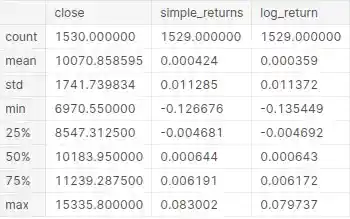
We call Pandas DataFrame describe method to generate descriptive statistics. The output of this method will provide detailed statistics in the form of mean, standard deviation, median, and quartiles.

data.describe()

The main advantage of log returns is that we can easily aggregate them across time, unlike simple returns. For instance, the log return for a year is the sum of the log returns of the days within the year. Additionally, log returns are symmetric around 0, and log return values can range from minus infinity to plus infinity. whereas simple returns' downside is limited to -100%, a negative movement of -25% (movement from 100 USD to 75 USD) does not reverse the losses by going +25% (75 USD to 93.75 USD).

Realized Volatility

Volatility plays an important role in trading and financial model forecasting. Next to directly modeling high–frequency returns, intra–day returns are also used to construct lower–frequency daily volatility measures, known as realized volatility. The application of volatility has tremendously increased due to the availability of high-frequency data and computational resources.

Layman’s definition: Realized volatility is the magnitude of daily price movements, regardless of direction, over a specific period.

Technical definition: Realized volatility is the daily standard deviation of log returns of an underlying asset, index, instrument, security, or ETF over a defined period with an assumed mean of zero.

Traders and data scientists use "realized volatility" to assess the predictive performance and adequacy of existing models and strategies due to our ability to observe the metric's non-latent character. Realized volatility is a particularly powerful indicator of price risk and its dynamics.

The formula for realized volatility is: $formula for realized volatility$

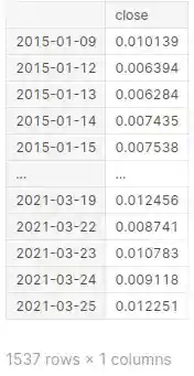
In Python, we create a function that calculates realized volatility with the help of the numpy functions sqrt and sum and pandas groupby and agg.

def realized_volatility(series):
    series = np.log(series).diff()
    return np.sqrt(np.sum(series**2))
df.groupby(df.index.date).agg(realized_volatility)

Realized Variance

Andersen and Bollerslev (1998) have suggested an ex-post intra-day volatility measure based on the sum of the squared intra-day returns. This concept is now known as "realized variance," and this is an ex-post observable measure.

$Realized variance formula$

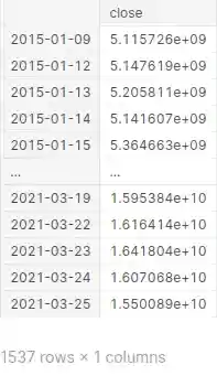
def realized_variance(series):
    return np.sum(series**2)
df.groupby(df.index.date).agg(realized_variance)

Summary

Using financial returns instead of prices allows us to measure and compare all financial instruments and assets. In Pandas, we calculate simple returns with an in-built pandas function called pct_change that calculates percentage change and use numpy's log to calculate log returns. The main advantage of log returns is that we can easily aggregate them across time, unlike simple returns. Log returns are symmetric around 0, and log return values can range from minus infinity to plus infinity. Whereas, simple returns' downside is limited to -100%, a negative movement of -25% (movement from 100 USD to 75 USD) does not reverse the losses by going +25%. (75 USD to 93.75 USD).

Simple returns vs log returns

Realized Volatility

Realized Variance

Summary

References and Related Posts