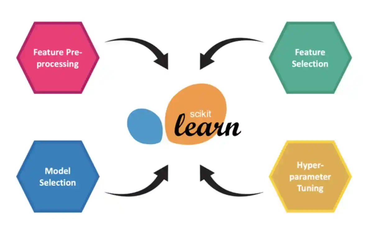
Simple sklearn ensemble machine learning

This post is a write up on sklearn ensemble pipeline for multiple target columns using traditional and established libraries such as numpy, pandas, scipy and sklearn. This post further extends article on sklearn pipeline for time-series data.

Some of the ideas for this post came from researching for machine learning competition Sound the Alarm 2 for Australian based platform Unearthed, where Dspyt team took 10th place on a private leader-board. The company is very strict about the data and code that they provided. You can try the platform in Evergreen Challenges.

Loading Libraries

First we need to load libraries, but our choice is limited to only well-established python libraries such as pandas, numpy and sklearn.

import numpy as np
import pandas as pd
from sklearn.tree import DecisionTreeRegressor

Loading data and hard code the tags

Next, in this example we have a single set of targets and input dataframes. In addition, we explicitly include the names of inputs and target columns under the variables input_tags and target_tags, respectively

inputs = pd.read_csv("/kaggle/input/sound-the-alarm2/public.csv")
targets = pd.read_csv("/kaggle/input/sound-the-alarm2/public.targets.csv")

Preprocessing and separating data into train and test

The preprocessing function aggregates unstructured data into time periods and tags.

def rolling(df, window, step):
    count = 0
    df_length = len(df)
    while count < (df_length - window):
        yield count, df[count:window+count]
        count += step

def preprocess(alarms, labels=None):

    alarms = alarms[alarms.major_down_time==False].drop(columns=['major_down_time'])
    #count frequencies
    t = alarms.groupby(['day', 'tag']).count().rename(columns={'date':'freq'}).reset_index()

    # add an empty row for all columns so we always get the same shape output
    t = t.append(pd.DataFrame({'day':[pd.to_datetime(alarms.date.values[0]).date()]*len(input_tags),'freq':[0]*len(input_tags), 'tag':input_tags}))
    X = pd.pivot_table(t, values='freq', columns='tag', index='day', aggfunc=np.sum).reset_index()

    # ensure the columns are in the same order
    X=X[['day'] + input_tags]
    x=dict()

    # For model input we will take 30 days of history for every row IE 3 dimensions
    # (sample_day, history date, column)
    # then flatten to 2 dimensions using date
    # (sample day, datecolumn)

    for offset, window in rolling(X, 30, 1): # prepare the X input
        d = window.tail(1).day.values[0]
        if d in labels[labels.window=='7 day'].date.values : # make sure we have a label for the date
            x[d]=window.drop(columns=['day']).fillna(0)

    inputs = [x[y] for y in x]
    inp = np.array(inputs)
    X = inp.reshape((inp.shape[0],inp.shape[1]*inp.shape[2])) # flatten to one row per day

    target1 = labels[(labels.window=='7 day') & labels.date.isin(x)].fillna(0)
    target2 = labels[(labels.window=='8-14 day') & labels.date.isin(x)].fillna(0)
    target3 = labels[(labels.window=='15-21 day') & labels.date.isin(x)].fillna(0)
    return X, x.keys(), target1[target_tags], target2[target_tags], target3[target_tags]

In this article the data has a significant reliance on the temporal dimension, therefore it is not the best practice to split data randomly into test and train. Hence, we put 80% of the first observations into train and 20% of the latest observations into a test data split.

X,dates,y1,y2,y3 = preprocess(inputs,targets)
X_train, X_test = X[:int(X.shape[0]*0.8)], X[int(X.shape[0]*0.8):]
dates_train, dates_test = list(dates)[:int(len(dates)*0.8)], list(dates)[int(len(dates)*0.8):]

sklearn ensemble model

To predict the labels for three columns we create an ensemble class that fits a separate decision tree model and combines individual predictions.

class  EnsembleModel:

    def __init__(self):
        self.models = dict()
        self.models['model1'] = DecisionTreeRegressor(random_state=1)
        self.models['model2'] = DecisionTreeRegressor(random_state=1)
        self.models['model3'] = DecisionTreeRegressor(random_state=1)

    def fit1(self, X, y):
        self.models['model1'].fit(X, y)

    def fit2(self, X, y):
        self.models['model2'].fit(X, y)

    def fit3(self, X, y):
        self.models['model3'].fit(X, y)

    def _predict(self,model_name, inp_X, dates):
        preds = self.models[model_name].predict(inp_X)
        preds = pd.DataFrame(dict(zip(target_tags,preds.T)))
        preds['date']=dates
        return preds

    def _predict_all(self,inp_X, dates):
        p1 = self._predict('model1',inp_X,dates)
        p2 = self._predict('model2',inp_X,dates)
        p3 = self._predict('model3',inp_X,dates)
        p1['window']=['7 day']*len(p1)
        p2['window']=['8-14 day']*len(p2)
        p3['window']=['15-21 day']*len(p3)
        return pd.concat([p1,p2,p3]).reset_index(drop=True)

    def predict(self, inp_X, dates):
        return self._predict_all(inp_X, dates)

Predict and score the predictions

In this section we initialize the ensemble model and fit each individual model to estimate predictions.

models = EnsembleModel()
models.fit1(X_train, y1[:167])
models.fit2(X_train, y2[:167])
models.fit3(X_train, y3[:167])

pred = models.predict(X_test, dates_test)

Moreover, we also build a scoring function that penalizes inaccurate predictions.


def scoring(gt, pred):
    gt['date']=pd.to_datetime(gt.date)
    pred['date']=pd.to_datetime(pred.date)

    gt = gt.set_index(['window','date'])

    pred = pred.set_index(['window','date'])
    m = gt.join(pred, how='inner', rsuffix='_pred')

    p_cols  = [c+"_pred" for c in target_tags]
    gt = m[target_tags].values
    pred = m[p_cols].values
    correct = np.bitwise_and(gt>0,pred>0).sum()
    incorrect = np.bitwise_and(gt==0,pred>0).sum()
    return correct - (incorrect/2)

scoring(targets, pred)

Summary

In this example we demonstrated how to combine machine learning functions into a pipeline. We used preprocessing function that cleans and aggregates data. Besides, we built sklearn ensemble model that fits individual models for three targets and predicts all the labels. Finally, we scored the predictions with the help of custom scoring function.

The areas for improvement are adding more features and improving the prediction models. Furthermore, we could use GridSearch and K-Folds cross-validator to estimate the necessary features and hyper parameters.